Extrapolation and House Price Cycles

by Michael Hatcher

Empirical evidence shows that house price busts are less frequent than equity price busts, but last about twice as long, with severe consequences for the macroeconomy. In a typical house price bust, the economy loses around 10% of GDP, with both consumption and investment taking a hit. It is not surprising, therefore, that housing and the macroeconomy is high on policymakers’ agenda.

In my Rebuilding Macroeconomics project I have developed a joint model for understanding house price booms and busts and their implications for the macroeconomy. The model has two parts: a housing market model in which investors differ in their levels of optimism about future house prices; and a macroeconomic model that is connected to the housing market through the wealth that investors accumulate – or lose – as a result of their housing transactions.

The housing model has two key features. First, homebuyers are speculative investors who buy houses not just for ‘living in’ but in anticipation of capital gains. Investors may borrow to finance house purchases but cannot default on the loan repayment. Second, cognitive limitations prevent investors from having rational expectations, but they attempt to maximize returns by switching to heuristics that performed well in the recent past. Some of these heuristics, or ‘rules of thumb’, are based on fundamentals such as interest rates; others are extrapolative, based on recent trends.

Extrapolators buy when prices have been rising and withdraw when the price trend turns negative.

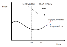
Differently to current approaches, investors may choose between multiple extrapolative predictors associated with different levels of optimism about future prices. This feature of the model, which I call endogenous extrapolation, has important implications; see Figure 1.

Fig . 1 – Myopic vs long extrapolative forecasts

A key feature of the model is that it generates persistent house price booms and busts. Figure 2 shows the response of house prices when the model is given initial values like the early stages of a price boom. After these initial periods, the level of house prices is endogenously determined by the model. The right-hand panel of Figure 1 shows the resulting price returns and the fraction of ‘optimistic investors’ who were anticipating future price increases.

House prices peak in period 8 and fall to a trough in period 16. The boom is helped by the strong initial demand of myopic extrapolators; however, their optimism soon wanes, and it is the demand of long extrapolators that keeps price increases going. This dynamic is consistent with Keynes' view that longer term expectations play a central role in speculative asset markets; and Karl Case and Robert Shiller have argued, using survey evidence, that such expectations were crucial in driving and sustaining the U.S. housing boom. Once prices pick up, fundamental investors exit the market, believing the high valuation of housing is not justified; hence, they remain off the `housing ladder' until prices fall. The boom turns to bust because fundamentalists are a drag on demand and the enthusiasm of extrapolators falls as house price increases fail to live up to expectations.

Fig. 2 – Boom, bust and optimism

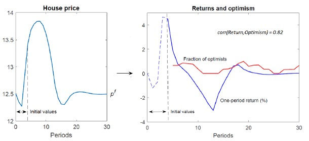
The cyclical house price dynamics in Figure 2 are protracted due to endogenous changes in optimism (see right panel). Investors become more optimistic during house price booms, and the resulting increase in demand pushes up prices. When the boom later turns to bust, pessimism sets in and hence the recovery in prices does not happen immediately.

This dynamic whereby changes in optimism are both a cause of and a response to price changes helps the model to generate a strong correlation between house price returns and investor optimism, as empirically supported in U.S. data. The model does well on this score because it generates waves of optimism that roughly coincide with house price peaks and troughs.

Given a working model of house prices, the question is: how to connect this to the macroeconomy?

Most work in macroeconomics has focused on the collateral channel, whereby an increase in house prices allows households to borrow more. I set out a model with a simpler wealth channel in aggregate demand. When house prices rise, wealth increases and households feel richer, consuming more as a result. A fall in house prices has the opposite effect.

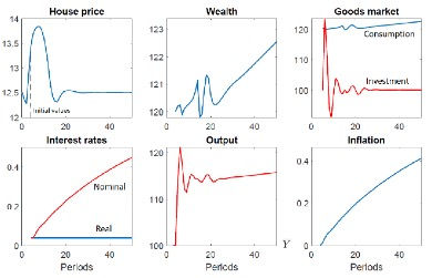
Figure 3 illustrates the impact of a housing boom and bust on aggregate wealth and macro variables, under the assumption that there is no monetary policy response through interest rates. We see that the increase in house prices raises consumption and output. Wealth and consumption take a sizeable hit when boom turns to bust, falling below their starting values. Ultimately, however, wealth recovers and continues an upward trend. As a result, the long run impact of the housing boom is expansionary: output ends up higher than it would otherwise have been.

It turns out that the long run impact on output hinges on wealth at the start of the boom. If wealth is sufficiently high the housing boom is expansionary as in Figure 3; however, if wealth falls below a critical threshold, this result is reversed. The reason is that if wealth is high investors then can buy with little or no borrowing, so that their wealth will grow provided house prices increase. For those lucky enough to buy housing without borrowing they have a cushion: any wealth not invested in housing is saved in bonds, and these (safe) returns may offset wealth losses if house prices fall.

However, if wealth is relatively low, most of the population will be forced to borrow to buy housing, in which cases they must repay with interest. If house prices rise rapidly this presents no problems. But if house price growth slows or enters negative territory they are in dire straits: capital gains on housing will not finance the debt repayments and hence wealth will fall, taking consumption and output with it. Note that our investors do not anticipate this predicament since their housing decisions are driven by their overly optimistic beliefs.

Figure 3 – Housing boom and macro variables: no interest rate response

Now consider a monetary policy response. Suppose that, following the advice of some economists, monetary policy ‘leans against the wind’ of house price increases by raising interest rates in response to house price growth. We show two such responses in Figure 4, along with the benchmark case of no monetary policy response; here starting wealth is at a more modest level than in Figure 3.

Figure 4 – Interest rate response to the housing boom

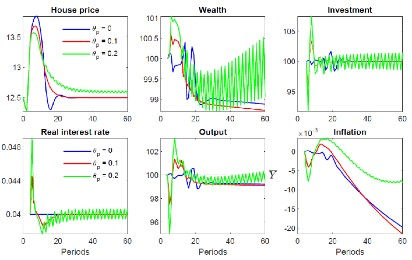
The top left panel shows that responding to house prices reigns in the boom somewhat, as well as preventing a bust in which house prices fall below their starting value. The more conservative response to house price growth (red line) leads to a similar long run impact to no response but avoids large fluctuations in wealth and output after the boom ends. The stronger response (green line) does well on average, and has wealth and output rising in the long run, unlike no response.

Unfortunately, this case is characterized by persistent (periodic) fluctuations in house prices and macro variables and has house prices permanently overvalued (top left panel). Moreover, stronger interest rate responses than this quickly cause house prices to collapse completely.

In short, the model warns us that ‘leaning against the wind’ of house price increases is a dangerous game. Does macro-prudential policy do any better? Here the results are more mixed: a cap on loan-wealth ratios is similarly risky to an interest rate response as this seems to produce highly unstable dynamics that warrant further investigation. However, a limit on house purchases per investor is as an effective (and equitable) stabilization tool. For a more detailed discussion of these policies see my Rebuilding Macroeconomics working paper.